
Fundamental steps in preparing data to model demand for your food products
It has never been more critical for food companies to leverage data to wring out every morsel of operational efficiency in order to manage costs.
As inflation rages, food and beverage manufacturers are facing price spikes in ingredients, packaging, and transportation. Reliably predicting food sales is a crucial first step in aligning production planning to consumer demand while simultaneously reducing waste.
In this piece, we will walk through the 3 key steps you need to consider when preparing your data to build demand prediction models. We will see how to eliminate data silos by connecting to all of your organization’s data sources regardless of their format or location. We will also explore best practices for time series forecasting, such as preparing targets for prediction, and what to do about pesky missing data and outliers.
These are the same steps we followed while successfully building an automated forecasting system for a commercial baker.
By the time you finish this piece, you will know how to properly import and prepare your data to predict demand for your food products without writing a single line of code. You can refer to our previous post to learn how to install and set up the free low-code KNIME Analytics Platform here.
If you want to become the forecasting guru for your food brand, follow along with our bi-weekly series as we demystify demand prediction for food and beverage manufacturing.
Step #1: Blend Your Data Silos
One of the great things about KNIME is how easy it is to connect and blend all of your data sources no matter how many there are or where they live.
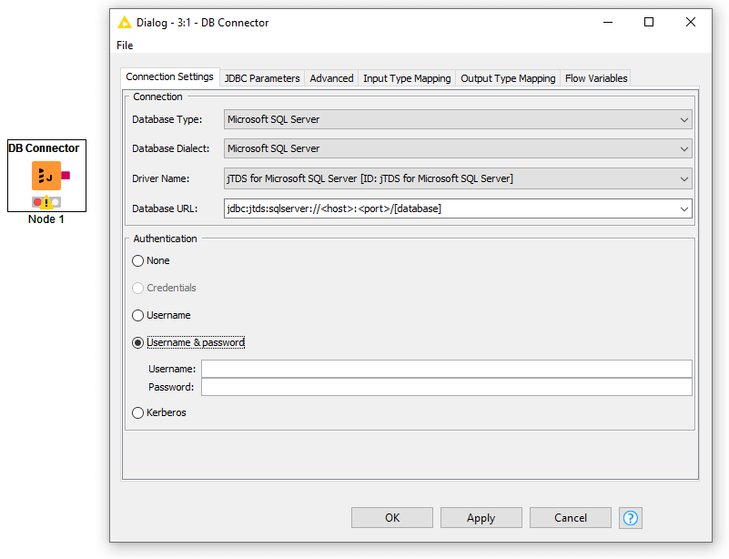
A simple search for “connector” under file → install KNIME Extensions [Figure 1], will show a long list of data connectors available for common file formats, cloud providers, and databases. If you can’t find your source system listed, a generic DB Connector node will connect to most databases using a JDBC driver. Once installed, you will find these connector nodes listed in the DB category in the Node Repository, along with many nodes for reading, cleaning, and writing data to and from your systems. [Figures 2, 3].
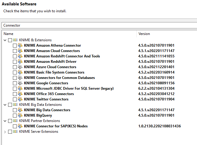
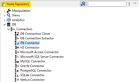
These data connectors allow for the systematic destruction of data silos by automatically integrating and blending all data sources.
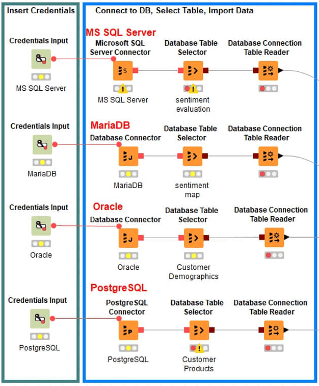
You can now connect to many common ERP, MRP, and WMS systems used by food manufacturers to manage production, materials, and inventory, respectively. These systems often live in databases located on-premises, on the cloud, or in a combination of the two. With KNIME, you can easily query the data you need, blend it with an unlimited number of data sources, and transform your data in minutes using repeatable and self-documenting visual programming workflows.
Figure 4 shows an example where four separate database platforms were blended to import various customer data tables, from four separate databases, for analysis onto a single visual workflow.
Step #2: Prepare Your Time Series Data
Granularity vs. Seasonality
Given the transactional nature of food & beverage sales, an important time-based pattern to consider is the granularity of data needed to predict demand for your products.
By granularity is meant: do you need daily, weekly, monthly, or yearly data for your forecasts? This choice can have a great effect on the accuracy of your model due to possible seasonal fluctuations in consumer demand as well as promotional activities throughout the year for many food products.
As a simple example, demand for ice cream is highly seasonal, thus the aim for an ice cream manufacturer with limited capacity should be to predict demand and plan total production for each seasonal period. In this case, aggregating sales data at a yearly level of granularity would be insufficient to highlight the seasonal effects in the model,as ice cream sales peak during summer months. Therefore, if data is being captured on an hourly, daily, or weekly basis, aggregating it to monthly would be necessary.
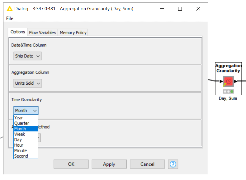
This can be easily done in KNIME using the Aggregation Granularity component. Simply select your Date-time column, the target prediction column you want to aggregate, and the level and type of aggregation.
In this example, we are simply aggregating the column we want to predict (units of ice cream sold), from its original hourly data, to month-level using the sum function [Figure 5].
Timestamp Alignment
Once you’ve determined the time-based granularity of your models, the next step is to align the timestamps in your data.
This simply means that your data must have an unbroken sequence of time-based entries. Time-series demand forecasting relies on previous entries to predict future transactions, so missing time entries are not allowed.
Fortunately, KNIME makes aligning time-based forecasting data effortless using the Timestamp Alignment component. [Figure 6].
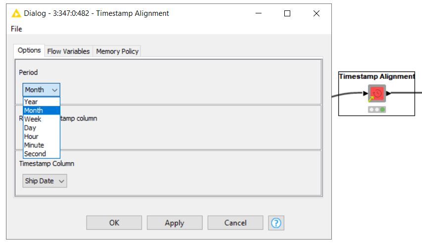
By simply selecting the period (e.g. monthly), the Timestamp Alignment component will create an entry for every necessary entry in your dataset.
If there are any missing entries in your data, they will now appear for any previously missing time-based transactions. You will now have timestamped entries with blank values for your target variable (volume or units sold, for instance). Therefore, the next step is handling missing values.
Fortunately, KNIME makes handling missing data easy as well.
Step #3: Handle Missing Data & Outliers
Missing Data
Now that you’ve blended your data sources together and prepared your time series data, the next step is to handle missing values and outliers.
These missing values might be due to a lack of sales transactions on a given day (e.g. weekends, holidays), or seasonal fluctuations in demand for your food products. Regardless of the reason, time-series forecasting models will not handle missing data well, so it is important to replace missing data with substitute values (a process known as imputation).
Luckily again, KNIME makes this process seamless thanks to the Missing Values node [Figure 7].
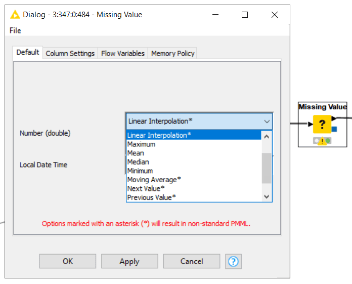
By simply choosing one of the many imputation methods provided, you can make sure that your imputed values closely match expected values. For example, using a moving average, mean, or linear interpolation, the substitute values will track closely to what would be expected for that given transaction.
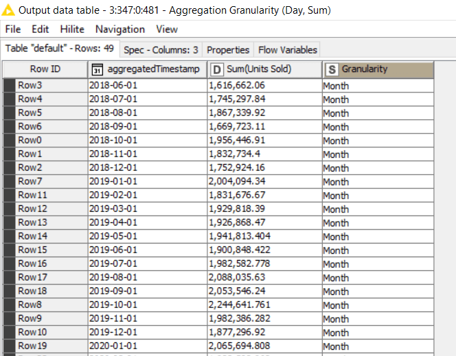
The final output would contain one aggregated record for every chosen period as shown in Figure 8.
Outliers
An outlier is a data point that falls outside an expected range.
Outliers can be caused by any number of reasons including, erroneous data entry, unforeseen spikes in demand for food products, or even natural variations. Whatever the cause, ignoring outliers in your data can be dangerous to demand forecasts. The process of fixing them is called ‘outlier correction.’
Similar to imputing missing data, the way to correct outliers is by replacing them with a more typical value.
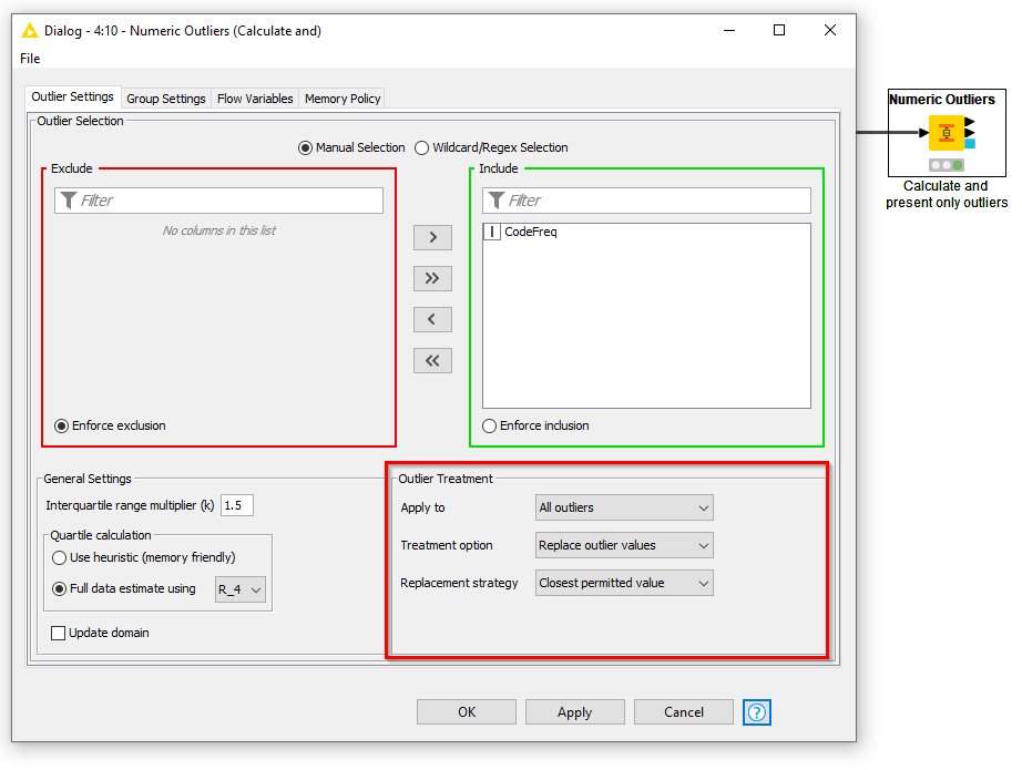
Once again, KNIME comes to the rescue by making this process easy with the Numeric Outlier node [Figure 9]. The node first detects outliers using an interquartile range (the middle 50% of values), and applies the closest permitted value within that range to the outlier. Alternatively, it can remove outliers entirely from a dataset, but this is not recommended without clearly understanding what caused the outlier in the first place.
TL;DR
- Demand forecasting is an important skill for food companies to master in order to align production to consumer demand and drive efficiency and reduce waste.
- The first step in preparing data for demand forecasting is to blend all required data sources on a single visual workflow for processing.
- The second step is preparing your data for time series analysis by selecting your granularity, aggregating the target value, and aligning timestamps.
- The third step is handling missing values and outliers to ensure your time series demand forecasting model works as expected.
Resources
- The KNIME Getting Started Guide: https://www.knime.com/getting-started-guide
- KNIME’s own self-paced courses: https://www.knime.com/knime-self-paced-courses
- The KNIME Starter Kit Video Series: https://youtube.com/playlist?list=PLz3mQ6OlTI0Ys_ZuXFTs5xMJAPKBmPNOf
Share the Love
If you enjoyed this post, please leave a comment below, share on your social networks, or share it with a colleague who can benefit from it.
➼ ARE YOU GOING TO IBIE?
LET’S CONNECT!