Build powerful Demand Forecasting solutions with KNIME Analytics Platform
The first step in building any demand forecast model in food manufacturing is to connect to your data sources.
In this post we will walk through the 5 steps you need to install and configure the free KNIME no-code analytics platform to properly connect and prepare your data for exploration, visualization, and time series analysis.
Whether your data lives in an ERP or MRP system, a data warehouse, or just plain old Excel files, these initial steps are critical in getting your demand forecasting right, and will spare you many hours of frustration later. By the time you finish this piece, you will learn how to properly configure KNIME in order to load your data for demand forecasting.
These are the same steps we followed while successfully building an automated forecasting system for a commercial baker.
Step #1: Install KNIME
You’ll first need to install the free KNIME desktop platform.
Don’t let the price tag fool you: despite being completely free, it is not a watered-down version of the platform. In fact, KNIME desktop is full-featured, containing over 4000 nodes with which to build your data solutions in modular, visual workflows.
The video below will walk you through the steps you need to quickly and easily install KNIME:
Step #2: Install Python
Why do we need Python?
KNIME is a code-free, drag-and-drop analytics platform. However, that doesn’t mean that it can’t play nice with popular data science programming languages such as R and Python.
In fact, it is often necessary to integrate these languages alongside KNIME in order to take advantage of popular extensions and features. Demand forecasting is one instance where we can take advantage of custom components for time series analysis written in Python.
To do that we’ll need to install Python on our machine. Don’t worry, we will not be programming in Python in this course.
First visit and download the Anaconda Python distribution from Continuum Analytics.
Simply select your operating system, download and run the executable file. That’s it! You now have the Python programming language installed on your machine. Next, we need to manage your Python installation on KNIME so that it knows where it is and which version you are using.
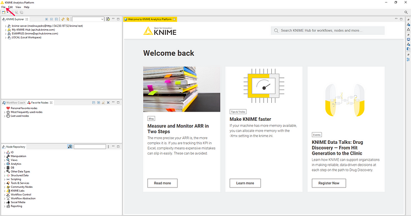
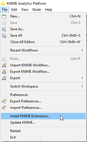
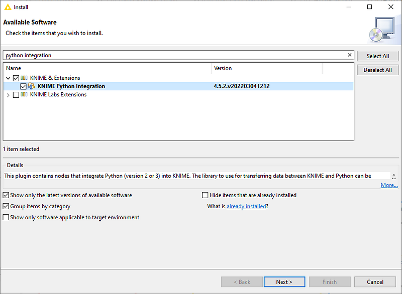
Step #3: Install the KNIME Python Integration
Now that you’ve installed KNIME and Python on your machine, open KNIME and go to file → install KNIME Extensions and search for KNIME Python Integration [Figures 1, 2, 3].
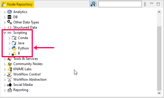
Once installed and configured, you will find the Python in your Node Repository [Figure 4].
Step #4: Manage your Python Environment
- With the Python Integration installed, go to the Python Preference page located at File → Preferences. Select KNIME → Python from the left panel. [Figure 5]
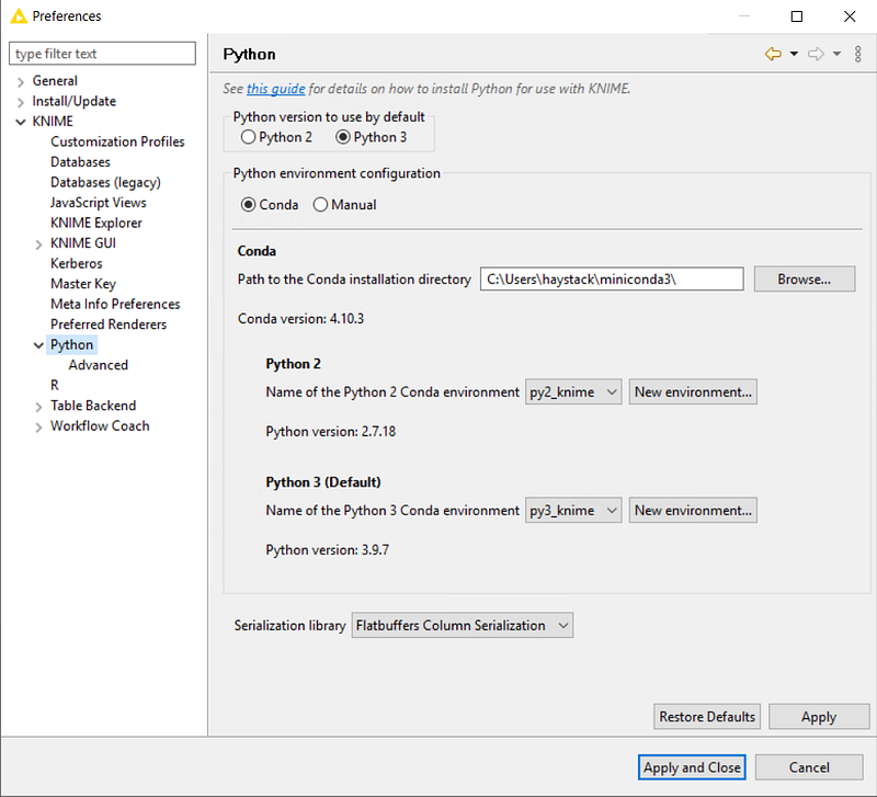
2. Now select Conda under Python environment configuration and provide the path to your installation folder (in Windows for example it is C:\Users\<your-username>\Anaconda3\, for Mac: /Users/<your-username>/Anaconda3, and Linux: /home/<your-username>/Anaconda3)
3. Choose which Conda environment is to be used for Python 2 and Python 3 by selecting it from the drop-down box.
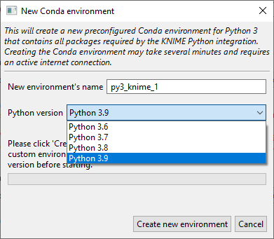
4. If you do not have an environment available, click ‘New environment,’ give it a name, and click ‘Create new environment’
For a more thorough explanation of the Python installation process in KNIME, please refer to the following document:
KNIME Python Integration Guide
Step #5: Access the Time Series Components
The final step is accessing the time series analysis components that we will be using to build our Demand Forecast model.
Time series components encapsulate functionality written in a Python script within a graphical interface (which is why we installed Python in the first place). They function just like regular nodes in that you can drag and drop them onto a workflow. They also have a dialog with options to configure their performance.
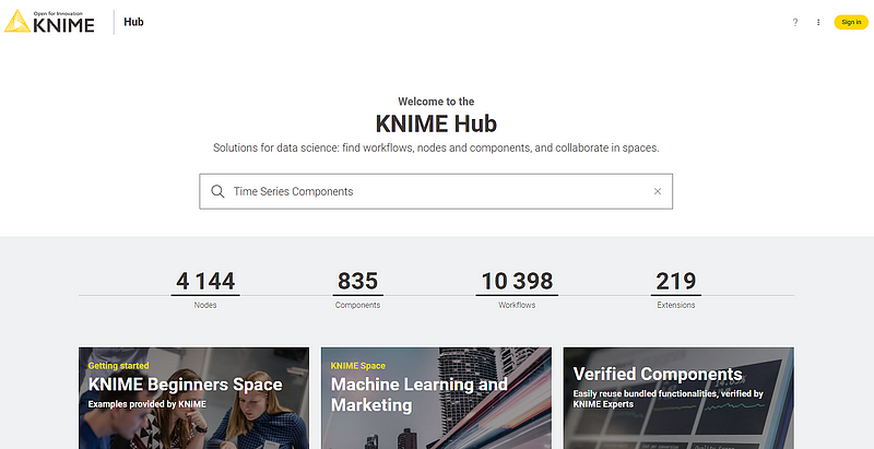
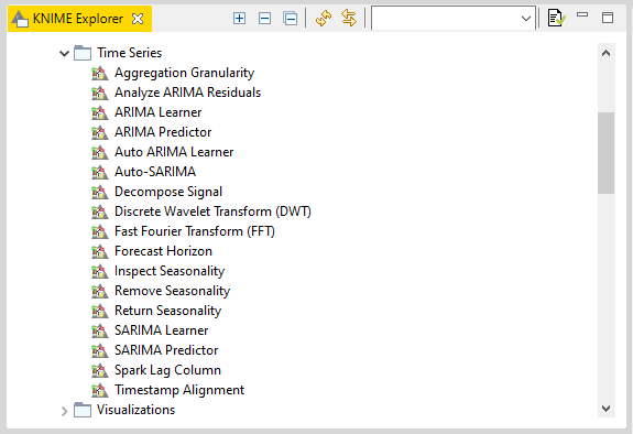
These components can be easily accessed either through the KNIME hub (hub.knime.com) or the EXAMPLES server directory within KNIME desktop [Figures 7, 8].
That’s it! You are now all set and ready to begin building your own Demand Forecast model without writing a single line of code!
Next time, we will look at how we load, clean, and explore data.
For now, explore the following resources that provide a gentle introduction to the KNIME analytics platform to help you learn your way around:
- The KNIME Getting Started Guide: https://www.knime.com/getting-started-guide
- KNIME’s own self-paced courses: https://www.knime.com/knime-self-paced-courses
- The KNIME Starter Kit Video Series: https://youtube.com/playlist?list=PLz3mQ6OlTI0Ys_ZuXFTs5xMJAPKBmPNOf
Share the Love
If you enjoyed this post, please leave a comment below, share on your social networks, or share it with a colleague who can benefit from it.
➼ ARE YOU GOING TO IBIE?
LET’S CONNECT!